01-intro-to-r

Author

Professor Shannon Ellis

Published

October 3, 2023

Introduction to R

[ad] Computing Paths

[ad] The Basement

[ad] CALPIRG

APPLY NOW: Protect the environment and make social change

CALPIRG Students is a student organization here that works to protect the environment, make college more affordable, and promote civic engagement. Last Fall we helped nearly 10,000 students register to vote in California and got the UCs to release new policy to phase out single-use plastics to protect our oceans! SIGN UP TO HELP NOW

Now, we are working to tackle the biggest problem facing our generation - climate change. Coming off another record-setting summer of hot temperatures, it’s clear we need to take strong, swift action to reduce the impacts of climate change. That’s why we are building support from students across the state to call for 100% clean energy UC-wide - for cars, buses, buildings, lights, and more! Fill out this interest form to learn more!

As a volunteer or intern with CALPIRG you can:

Work with the media and help organize events like a Solar-Powered Concert and climate week of action

Increase voting accessibility and voter turnout in elections

Bring down the cost of textbooks

Protect wildlife like whales and sea otters in the Pacific

And more!

Q&A

Q: How are groups formed for the projects?
A: I form them randomly for the two case studies and students get to choose their own groups for the final project.

Q: I’m curious about what the workload would be like for the case studies.
A: We’ll discuss this when the time comes in detail but for now, students are presented with a lot of the starter code for the case studies. You and your group mates have to get teh code running, add explanations, and “extend” the case study, meaning add something meaningful onto what was presented.

Q: Will this course go into advanced topics in tidyverse?
A: We will certainly go beyond the basic dplyr verbs and cover multiple packages in the tidyverse, but we won’t be able to cover everything.

Q: Would it be possible to have access to the third Case Study just to work on our own time?
A: Yup! I’ll you all in the direction of OpenCaseStudies, which is a resource I’ll be using for 1 of the 2 case studies this quarter, and that we used for all case studies previously.

Q: How many homework assignments are there? Some slides said 3, some said 4.
A: Apologies. There are 3. (There were previously 4 but I removed one. Slides have been updated.)

Q: Could we just sit in for lectures? Can I keep watching lectures?
A: Yup - this would be fine, so long as everyone enrolled had a seat. And, the podcasts are open to anyone!

Q: If we decide to do our projects and homework locally, how can we download/install the packages necessary for it?
A: This is covered in your first lab!

Q: I’m generally curious on how the language R is used in real world settings after college. What are its specific uses and what are the better ways to learn the language to maximize its utility. Also, how does this language differ from python in the data science realm.
A: Great question that we’ll cover throughout the course. However, breifly here, R is most heavily used by individuals who do more statistics, who work in biology, psychology or economics, and/or who analyze data regularly.

Q: What is the advantage of using R over other programming languages to do data science tasks? How much is R used for data science in the real world?
A: Within the tidyverse and in RStudio, the advantage is the cohesiveness of the tools - once you gain familiarity you can often intuit how to use another tool in the tidyverse. R is used for data science across tons of companies; however, across industries. its use is not as widespread as Python.

Course Announcements

Due Dates:

Student survey “due” today 11:59 PM
Lab 01 due Friday (11:59 PM)
Lecture Participation survey “due” after class

Waitlist (Non)Update: Staff are seeing what options there are. A few people got an email from Kasey Chiang (k4chiang@ucsd.edu) to drop and then enroll. This is legitimate. Follow those instructions.

Agenda

Variables
Operators
Data in R
RMarkdown

Variables & Assignment

Variables are how we store information so that we can access it later.

Variables are created and stored using the assignment operator <-

first_variable <- 3

The above stores the value 3 in the variable first_variable

Note: Other programming languages use = for assignment. R also uses that for assignment, but it is more typical to see <- in R code, so we’ll stick with that.

This means that if we ever want to reference the information stored in that variable later, we can “call” (mean, type in our code) the variable’s name:

first_variable

[1] 3

Variable Type

Every variable you create in R will be of a specific type.

The type of the variable is determined dynamically on assignment.

Determining the type of a variable with class():

class(first_variable)

[1] "numeric"

Basic Variable Types

Variable Type	Explanation	Example
character	stores a string	`"cogs137"`, `"hi!"`
numeric	stores whole numbers and decimals	`9`, `9.29`
integer	specifies integer	`9L` (the `L` specifies this is an integer)
logical	Booleans	`TRUE`, `FALSE`
list	store multiple elements	`list(7, "a", TRUE)`

Note: There are many more. We’ll get to some but not all in this course.

logical & character

logical - Boolean values TRUE and FALSE

class(TRUE)

[1] "logical"

character - character strings

class("hello")

[1] "character"

class('students') # equivalent...but we'll use double quotes!

[1] "character"

numeric: double & integer

double - floating point numerical values (default numerical type)

class(1.335)

[1] "numeric"

class(7)

[1] "numeric"

integer - integer numerical values (indicated with an L)

class(7L)

[1] "integer"

lists

So far, every variable has been an atomic vector, meaning it only stores a single piece of information.

Lists are 1d objects that can contain any combination of R objects

mylist <- list("A", 7L, TRUE, 18.4)
mylist

[[1]]
[1] "A"

[[2]]
[1] 7

[[3]]
[1] TRUE

[[4]]
[1] 18.4

str(mylist)

List of 4
 $ : chr "A"
 $ : int 7
 $ : logi TRUE
 $ : num 18.4

Your Turn

Define variables of each of the following types: character, numeric, integer, logical, list

Put a green sticky on the front of your computer when you’re done. Put a pink if you want help/have a question.

Functions

class() (and View() & median()) were our first functions…but we’ll show a few more.

Functions are (most often) verbs, followed by what they will be applied to in parentheses.

Functions are:

available from base R
available from packages you import
defined by you

We’ll start by getting comfortable with available functions, but in a few days, you’ll learn how to write your own!

Helpful Functions

class() - determine high-level variable type

class(mylist)

[1] "list"

length()- determine how long an object is

# contains 4 elements
length(mylist)

[1] 4

str() - display the structure of an R object

str(mylist)

List of 4
 $ : chr "A"
 $ : int 7
 $ : logi TRUE
 $ : num 18.4

Coercion

R is a dynamically typed language – it will happily convert between the various types without complaint.

c(1, "Hello")

[1] "1"     "Hello"

c(FALSE, 3L)

[1] 0 3

c(1.2, 3L)

[1] 1.2 3.0

Missing Values

R uses NA to represent missing values in its data structures.

class(NA)

[1] "logical"

Other Special Values

NaN | Not a number

Inf | Positive infinity

-Inf | Negative infinity

Activity

What is the type of the following vectors? Chat about why they have that type.

c(1, NA+1L, "C")
c(1L / 0, NA)
c(1:3, 5)
c(3L, NaN+1L)
c(NA, TRUE)

Put a green sticky on the front of your computer when you’re done. Put a pink if you want help/have a question.

Operators

At its simplest, R is a calculator. To carry out mathematical operations, R uses operators.

Arithmetic Operators

Operator	Description
`+`	addition
`-`	subtraction
`*`	multiplication
`/`	division
`^` or `**`	exponentiation
`x %% y`	modulus (x mod y) `9%%2` is 1
`x %/% y`	integer division `9%/%2` is 4

Arithmetic Operators: Examples

7 + 6

[1] 13

2 - 3

[1] -1

4 * 2

[1] 8

9 / 2

[1] 4.5

Reminder

Output can be stored to a variable

my_addition <- 7 + 6

my_addition

[1] 13

Comparison Operators

These operators return a Boolean.

Operator	Description
`<`	less than
`<=`	less than or equal to
`>`	greater than
`>=`	greater than or equal to
`==`	exactly equal to
`!=`	not equal to

Comparison Operators: Examples

4 < 12

[1] TRUE

4 >= 3

[1] TRUE

6 == 6

[1] TRUE

7 != 6

[1] TRUE

Your Turn

Use arithmetic and comparison operators to store the value 30 in the variable var_30 and TRUE in the variable true_var.

Put a green sticky on the front of your computer when you’re done. Put a pink if you want help/have a question.

R Packages

Packages

Packages are installed with the install.packages function and loaded with the library function, once per session:

install.packages("package_name")
library(package_name)

In this course, most packages we’ll use have been installed for you already on datahub, so you will only have to load the package in (using library).

Data “sets”

Data “sets” in R

“set” is in quotation marks because it is not a formal data class
A tidy data “set” can be one of the following types:
- tibble
- data.frame
We’ll often work with tibbles:
- readr package (e.g. read_csv function) loads data as a tibble by default
- tibbles are part of the tidyverse, so they work well with other packages we are using
- they make minimal assumptions about your data, so are less likely to cause hard to track bugs in your code

Data frames

A data frame is the most commonly used data structure in R, they are list of equal length vectors (usually atomic, but can be generic). Each vector is treated as a column and elements of the vectors as rows.
A tibble is a type of data frame that … makes your life (i.e. data analysis) easier.
Most often a data frame will be constructed by reading in from a file, but we can create them from scratch.

df <- tibble(x = 1:3, y = c("a", "b", "c"))
class(df)

[1] "tbl_df"     "tbl"        "data.frame"

glimpse(df)

Rows: 3
Columns: 2
$ x <int> 1, 2, 3
$ y <chr> "a", "b", "c"

Data frames (cont.)

attributes(df)

$class
[1] "tbl_df"     "tbl"        "data.frame"

$row.names
[1] 1 2 3

$names
[1] "x" "y"

Columns (variables) in data frames are accessed with $:

dataframe$var_name

class(df$x)  # access variable type for column

[1] "integer"

class(df$y)

[1] "character"

Variable Types

Data stored in columns can include different kinds of information…which would require a different type (class) of variable to be used in R.

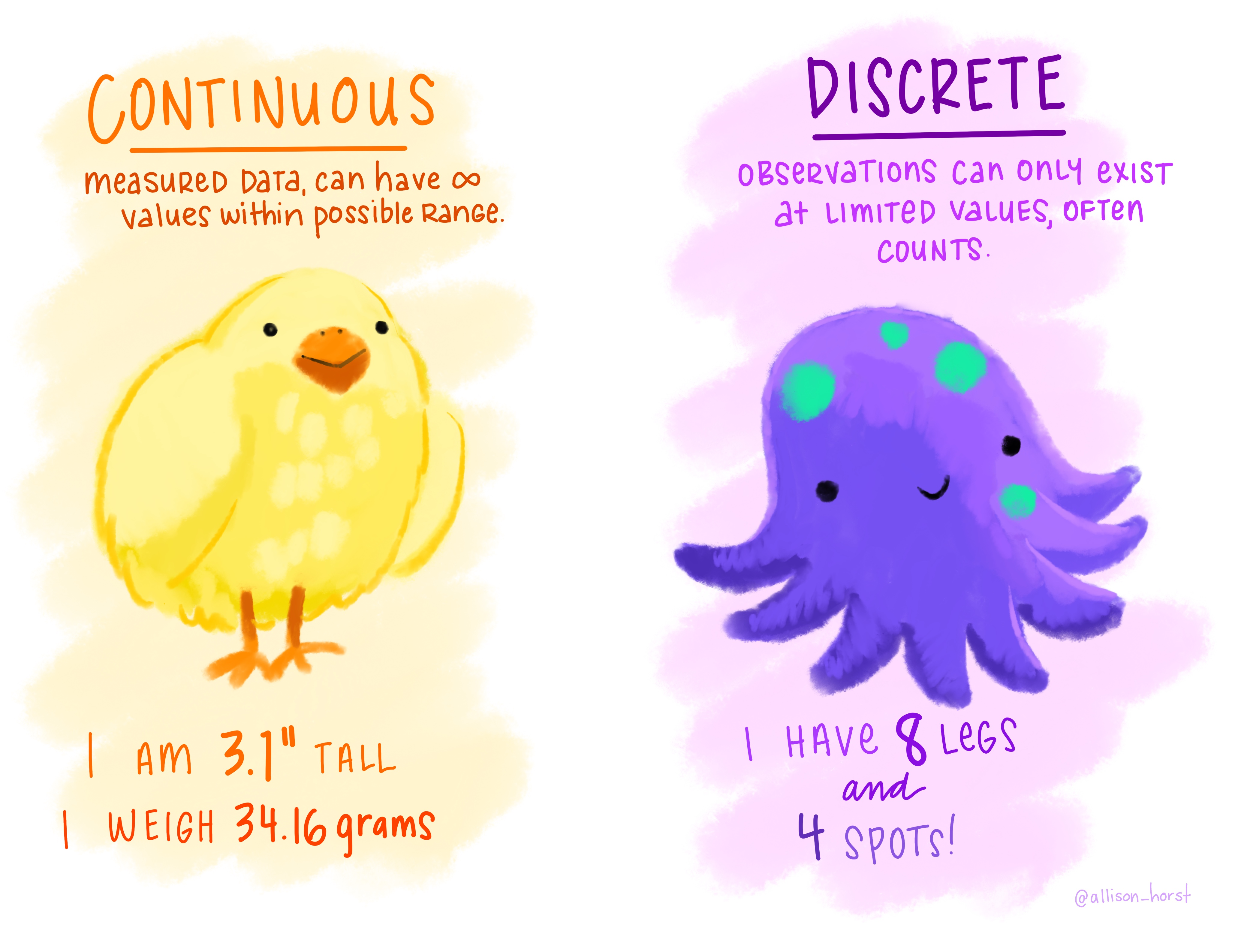
R Data Types:

Continuous: numeric, integer
Discrete: factors (we haven’t talked about these yet, but will today!)

Artwork by @allison_horst

Variable Types (cont.)

Sometimes data are non-numeric and store words. Even when that is the case, the data can be conveying different information.

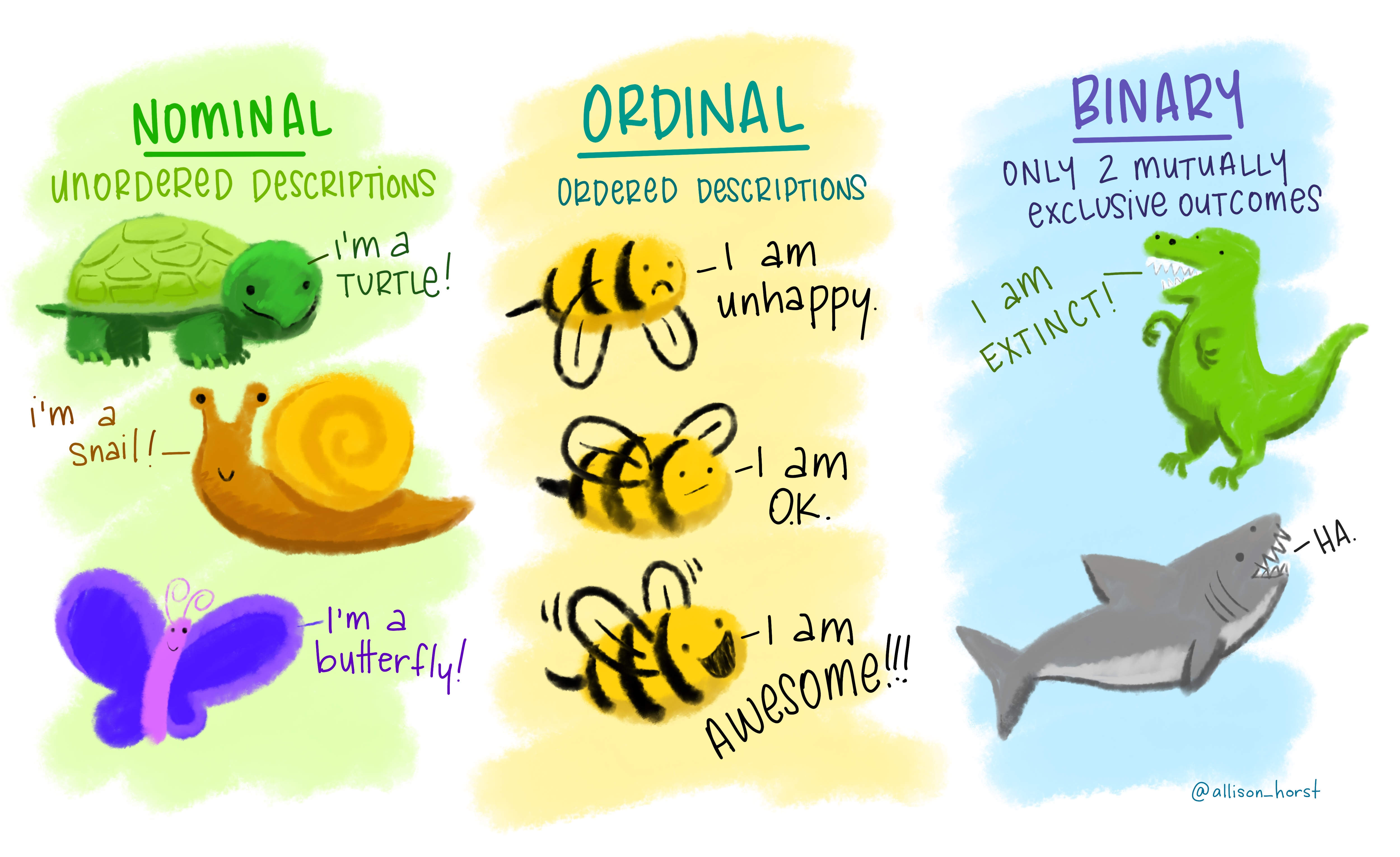
R Data Types:

Nominal: character
Ordinal: factors
Binary: logical OR numeric OR factors 😱

Artwork by @allison_horst

Example: Cat lovers

A survey asked respondents their name and number of cats. The instructions said to enter the number of cats as a numerical value.

🚨 There is code ahead that we’re not going to discuss in detail today, but we will in coming lectures.

cat_lovers <- read_csv("https://raw.githubusercontent.com/COGS137/datasets/main/cat-lovers.csv")

The Data

cat_lovers |>
  datatable()

The Question

How many respondents have a below average number of cats?

Giving it a first shot…

cat_lovers |>
  summarise(mean = mean(number_of_cats))

Warning: There was 1 warning in `summarise()`.
ℹ In argument: `mean = mean(number_of_cats)`.
Caused by warning in `mean.default()`:
! argument is not numeric or logical: returning NA

# A tibble: 1 × 1
   mean
  <dbl>
1    NA

💡 maybe there is missing data in the number_of_cats column!

Oh why will you still not work??!!

cat_lovers |>
  summarise(mean_cats = mean(number_of_cats, na.rm = TRUE))

Warning: There was 1 warning in `summarise()`.
ℹ In argument: `mean_cats = mean(number_of_cats, na.rm = TRUE)`.
Caused by warning in `mean.default()`:
! argument is not numeric or logical: returning NA

# A tibble: 1 × 1
  mean_cats
      <dbl>
1        NA

💡What is the type of the number_of_cats variable?

Take a breath and look at your data

glimpse(cat_lovers)

Rows: 60
Columns: 3
$ name           <chr> "Bernice Warren", "Woodrow Stone", "Willie Bass", "Tyro…
$ number_of_cats <chr> "0", "0", "1", "3", "3", "2", "1", "1", "0", "0", "0", …
$ handedness     <chr> "left", "left", "left", "left", "left", "left", "left",…

Let’s take another look

Sometimes you need to babysit your respondents

cat_lovers |>
  mutate(number_of_cats = case_when(
    name == "Ginger Clark" ~ 2,
    name == "Doug Bass"    ~ 3,
    TRUE                   ~ as.numeric(number_of_cats)))

Warning: There was 1 warning in `mutate()`.
ℹ In argument: `number_of_cats = case_when(...)`.
Caused by warning:
! NAs introduced by coercion

# A tibble: 60 × 3
   name           number_of_cats handedness
   <chr>                   <dbl> <chr>     
 1 Bernice Warren              0 left      
 2 Woodrow Stone               0 left      
 3 Willie Bass                 1 left      
 4 Tyrone Estrada              3 left      
 5 Alex Daniels                3 left      
 6 Jane Bates                  2 left      
 7 Latoya Simpson              1 left      
 8 Darin Woods                 1 left      
 9 Agnes Cobb                  0 left      
10 Tabitha Grant               0 left      
# ℹ 50 more rows

Always respect (& check!) data types

cat_lovers |>
  mutate(number_of_cats = case_when(
         name == "Ginger Clark" ~ "2",
         name == "Doug Bass"    ~ "3",
         TRUE                   ~ number_of_cats),
         number_of_cats = as.numeric(number_of_cats)) |>
  summarise(mean_cats = mean(number_of_cats))

# A tibble: 1 × 1
  mean_cats
      <dbl>
1     0.817

Now that we know what we’re doing…

cat_lovers <- cat_lovers |>
  mutate(number_of_cats = case_when(
         name == "Ginger Clark" ~ "2",
         name == "Doug Bass"    ~ "3",
         TRUE                   ~ number_of_cats),
         number_of_cats = as.numeric(number_of_cats))

… store your data in a variable (here we’re overwriting the old cat_lovers tibble).

Moral of the story

If your data does not behave how you expect it to, type coercion upon reading in the data might be the reason.
Go in and investigate your data, apply the fix, save your data, live happily ever after.

R Markdown

R Markdown: tour

[DEMO]

Before we move on…

What is the Bechdel test?

The Bechdel test asks whether a work of fiction features at least two women who talk to each other about something other than a man, and there must be two women named characters.

Concepts introduced:

Knitting documents
R Markdown and (some) R syntax

GitHub Setup

See this week’s lab…

Put a green sticky on the front of your computer when you’re done. Put a pink if you want help/have a question.

Giving the demo a go…

Navigate to the demo URL (on Canvas)
Accept the “assignment” (this is NOT graded)
Clone the repo
Edit the document
Knit the document
Push your changes

Try to play around with this after finishing your lab tomorrow!

Recap

Always best to think of data as part of a tibble
- This plays nicely with the tidyverse as well
- Rows are observations, columns are variables
What are the common variable types in R
- How do I create a variable of each type?
- When would I use each one?
Do I know how to determine the class/type of a variable?
Can I explain dynamic typing?
Can I operate on variables and values using…
- arithmetic operators?
- comparison operators?
What are dataframes/tibbles? and why are they useful?
What is the difference between installing and loading a package?
What are the components of an R Markdown file?