03-tidyr
Tidy Data with tidyr
[ad] Data Science Student Society
Join DS3 at their Fall General Body Meeting to learn more about the events they’re offering this quarter, open board positions for the year, and free food! It will be happening on Wednesday (10/11) from 6-8pm, at PC Ballroom West
Q&A
Q: Is it possible to integrate to github using other systems than datahub? Datahub has already been spotty for me in this course and is notorious for slumping at critical pts in the quarter.
A: Yup. The same steps can be carried out by downloading RStudio onto your computer and connecting it with GitHub.
Q: Should we write in the console or in the rmd file first when writing code?
A: Great question! I’d suggest starting in the Rmd file and editing there. That way you don’t have to copy+paste once you get it right. It’s already there.
Q: How do you take notes for coding classes? I know there are lecture notes available, but how would you recommend taking notes for this class?
A: I would recommend opening a blank Rmd each day for class and saving it with the lecture number. I’d keep notes and things I tried in that file. But, I wouldn’t copy+paste everything, since the other lecture notes are available.
Course Announcements
Due Dates:
- Lab 02 due Friday
- HW01 now available; due Monday (10/16; 11:59 PM)
- Lecture Participation survey open until Thursday
. . .
Notes:
- Lab01 scores and feedback posted
- Datahub: Launch RStudio (possible solution?)
- Staff office hours updated (see Canvas or website)
Student Comment
I have been struggling to grasp the material in the course. It feels like we are diving into the content in the labs, but I don’t even feel like I truly understand what I’m doing. It often seems like I’m just copying and pasting code from the website without a clear understanding of the bigger picture. I’m particularly stuck because I feel like I don’t have a solid grasp of the fundamental concepts of coding in R; it feels so new. I understand that the pace of the course may be challenging, but I think a bit more stronger focus on the foundational aspects of coding in R would greatly benefit students like me who are struggling with the content. I’m looking forward to the course and I hope I can grasp the content as we go through the next week. I’m concerned about learning the material and also how that may affect my grade.
. . .
Let’s see how y’all feel in a week. The first week can be a lot in this course. Often, students feel a lot more comfortable come week 3.
Student Survey
- 89% know Python; 15% know R; most (but not all!) have programmed before
- 64% feel confident about effective data science communication
- Reasons for taking course: learn R, add to resume, analyze data, improve data science skills
. . .
My favorite boring facts:
- I was actually born on my birthday
- i don’t like to eat eggs but my roommate loves them
- I like to have a midday nap.
- I can raise my eyebrows really well
- I eat peanut butter straight from the jar
- i have a jack russell terrier.. named jack (we weren’t feeling creative)
Suggested Reading
R4DS:
- Chapter 12: Tidy Data
- Chapter 13: Relational Data
Tidy Data
The opinionated tidyverse is named as such b/c it assumes/necessitates your data be “tidy”.
. . .
Tidy datasets are all alike, but every messy dataset is messy in its own way. —- Hadley Wickham
. . .
- Each variable must have its own column.
- Each observation must have its own row.
- Each value must have its own cell.
Source: https://r4ds.had.co.nz/tidy-data.html
Tidy or not?
❓ Given the rules discussed, is the cat_lovers dataset tidy?
cat_lovers <- read_csv("https://raw.githubusercontent.com/COGS137/datasets/main/cat-lovers.csv")Rows: 60 Columns: 3
── Column specification ────────────────────────────────────────────────────────
Delimiter: ","
chr (3): name, number_of_cats, handedness
ℹ Use `spec()` to retrieve the full column specification for this data.
ℹ Specify the column types or set `show_col_types = FALSE` to quiet this message.cat_lovers |> datatable(). . .
❓ Given the rules discussed, is the bike dataset tidy?
bike <- read_csv2("https://raw.githubusercontent.com/COGS137/datasets/main/nc_bike_crash.csv",
                  na = c("NA", "", "."))
ℹ Using "','" as decimal and "'.'" as grouping mark. Use `read_delim()` for more control.Rows: 5716 Columns: 54
── Column specification ────────────────────────────────────────────────────────
Delimiter: ";"
chr (44): AmbulanceR, BikeAge_Gr, Bike_Alc_D, Bike_Dir, Bike_Injur, Bike_Po...
dbl (8): FID, OBJECTID, Bike_Age, Crash_Hour, Crash_Ty_1, Crash_Year, Drvr...
dttm (1): Crash_Time
date (1): Crash_Date
ℹ Use `spec()` to retrieve the full column specification for this data.
ℹ Specify the column types or set `show_col_types = FALSE` to quiet this message.bike |> datatable()Warning in instance$preRenderHook(instance): It seems your data is too big for
client-side DataTables. You may consider server-side processing:
https://rstudio.github.io/DT/server.htmlSummary tables
❓ Which is a dataset? Which is a summary table?
Your Turn
There are four representations of the same data/information provided in the tidyr packages: table1, table2, table3, and the combination of table4a and table4b. Given what we’ve discussed, which is the best (tidiest) way to represent these data?
Put a green sticky on the front of your computer when you’re done. Put a pink if you want help/have a question.
Common issues
- One variable might be spread across multiple columns.
- One observation might be scattered across multiple rows.
. . .
Solution: pivoting!
Pivoting
For when some of the column names are not names of variables, but values of a variable…
table4a# A tibble: 3 × 3
country `1999` `2000`
<chr> <dbl> <dbl>
1 Afghanistan 745 2666
2 Brazil 37737 80488
3 China 212258 213766table4a |>
pivot_longer(c(`1999`, `2000`), names_to = "year", values_to = "cases")# A tibble: 6 × 3
country year cases
<chr> <chr> <dbl>
1 Afghanistan 1999 745
2 Afghanistan 2000 2666
3 Brazil 1999 37737
4 Brazil 2000 80488
5 China 1999 212258
6 China 2000 213766❓ Why are there backticks around the years? (Note: we have not discussed this yet)
For when an observation is scattered across multiple rows…
table2# A tibble: 12 × 4
country year type count
<chr> <dbl> <chr> <dbl>
1 Afghanistan 1999 cases 745
2 Afghanistan 1999 population 19987071
3 Afghanistan 2000 cases 2666
4 Afghanistan 2000 population 20595360
5 Brazil 1999 cases 37737
6 Brazil 1999 population 172006362
7 Brazil 2000 cases 80488
8 Brazil 2000 population 174504898
9 China 1999 cases 212258
10 China 1999 population 1272915272
11 China 2000 cases 213766
12 China 2000 population 1280428583table2 |>
pivot_wider(names_from = type, values_from = count)# A tibble: 6 × 4
country year cases population
<chr> <dbl> <dbl> <dbl>
1 Afghanistan 1999 745 19987071
2 Afghanistan 2000 2666 20595360
3 Brazil 1999 37737 172006362
4 Brazil 2000 80488 174504898
5 China 1999 212258 1272915272
6 China 2000 213766 1280428583❓ Why aren’t there quotes around column names here…but there were in pivot_longer? (Note: we have not discussed this yet.)
- wide data contains values that do not repeat in the first column.
- long format contains values that do repeat in the first column.
Both are good/helpful! We’ll return to this idea and discuss more during dataviz next week.
Briefly:
- wide data: analysis
- long data: plotting
Separating & Uniting
For when multiple pieces of information are stored in a single column…
table3# A tibble: 6 × 3
country year rate
<chr> <dbl> <chr>
1 Afghanistan 1999 745/19987071
2 Afghanistan 2000 2666/20595360
3 Brazil 1999 37737/172006362
4 Brazil 2000 80488/174504898
5 China 1999 212258/1272915272
6 China 2000 213766/1280428583table3 |>
separate(rate, into = c("cases", "population"))# A tibble: 6 × 4
country year cases population
<chr> <dbl> <chr> <chr>
1 Afghanistan 1999 745 19987071
2 Afghanistan 2000 2666 20595360
3 Brazil 1999 37737 172006362
4 Brazil 2000 80488 174504898
5 China 1999 212258 1272915272
6 China 2000 213766 1280428583…but…but…cases and population should be numeric…
table3 |>
  separate(rate, into = c("cases", "population"), convert = TRUE)
# A tibble: 6 × 4
country year cases population
<chr> <dbl> <int> <int>
1 Afghanistan 1999 745 19987071
2 Afghanistan 2000 2666 20595360
3 Brazil 1999 37737 172006362
4 Brazil 2000 80488 174504898
5 China 1999 212258 1272915272
6 China 2000 213766 1280428583Unite is the opposite…it combines data stored across multiple columns.
The general syntax is:
df |>
  unite(new_col, first_col, second_col)
Joins
If we look at table4a, it’s missing the population information. That’s stored in a separate table…table4b
table4b# A tibble: 3 × 3
country `1999` `2000`
<chr> <dbl> <dbl>
1 Afghanistan 19987071 20595360
2 Brazil 172006362 174504898
3 China 1272915272 1280428583…which is also in the “wide” format
. . .
…so we pivot both tables longer
tidy4a <- table4a |>
  pivot_longer(c(`1999`, `2000`), names_to = "year", values_to = "cases")

tidy4b <- table4b |>
  pivot_longer(c(`1999`, `2000`), names_to = "year", values_to = "population")

tidy4b
# A tibble: 6 × 3
country year population
<chr> <chr> <dbl>
1 Afghanistan 1999 19987071
2 Afghanistan 2000 20595360
3 Brazil 1999 172006362
4 Brazil 2000 174504898
5 China 1999 1272915272
6 China 2000 1280428583. . .
…but how do we get them into a single tidy dataset?
. . .
A join!
left_join(tidy4a, tidy4b)Joining with `by = join_by(country, year)`# A tibble: 6 × 4
country year cases population
<chr> <chr> <dbl> <dbl>
1 Afghanistan 1999 745 19987071
2 Afghanistan 2000 2666 20595360
3 Brazil 1999 37737 172006362
4 Brazil 2000 80488 174504898
5 China 1999 212258 1272915272
6 China 2000 213766 1280428583Source: R4DS
The Data: nycflights13
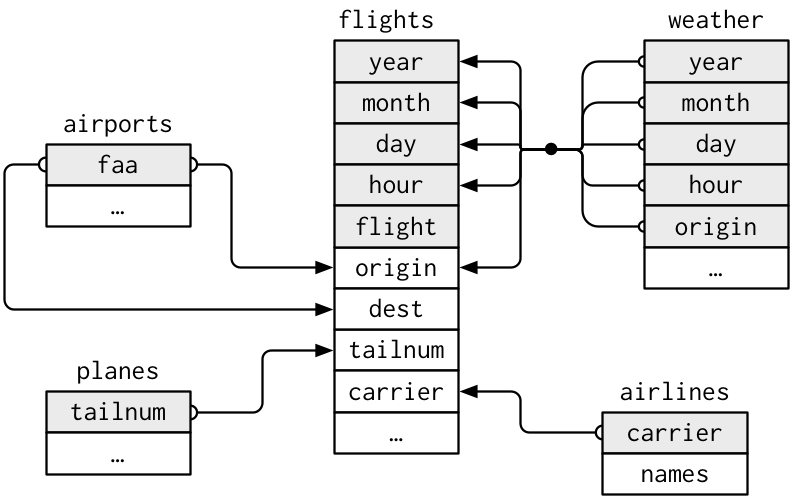
library(nycflights13)airlines: links airline to two letter codeairports: ID’ed by FAA codeplanes: ID’ed by tailnumairport: weather each hour; id’ed by two letter airport code
. . .
. . .
flightsconnects toplanesvia a single variable,tailnum.flightsconnects toairlinesthrough thecarriervariable.flightsconnects toairportsin two ways: via theoriginanddestvariables.flightsconnects toweatherviaorigin(the location), andyear,month,dayandhour(the time).
Mutating Joins
mutating joins - add new variables to a data frame from matching observations in another
. . .
For simplicity, we’ll work with only a handful of columns…
flights |>
  select(year:day, hour, tailnum, carrier) |>
  left_join(airlines, by = "carrier")
# A tibble: 336,776 × 7
year month day hour tailnum carrier name
<int> <int> <int> <dbl> <chr> <chr> <chr>
1 2013 1 1 5 N14228 UA United Air Lines Inc.
2 2013 1 1 5 N24211 UA United Air Lines Inc.
3 2013 1 1 5 N619AA AA American Airlines Inc.
4 2013 1 1 5 N804JB B6 JetBlue Airways
5 2013 1 1 6 N668DN DL Delta Air Lines Inc.
6 2013 1 1 5 N39463 UA United Air Lines Inc.
7 2013 1 1 6 N516JB B6 JetBlue Airways
8 2013 1 1 6 N829AS EV ExpressJet Airlines Inc.
9 2013 1 1 6 N593JB B6 JetBlue Airways
10 2013 1 1 6 N3ALAA AA American Airlines Inc.
# ℹ 336,766 more rowsThere is now a new column name…coming from the airlines data frame.
. . .
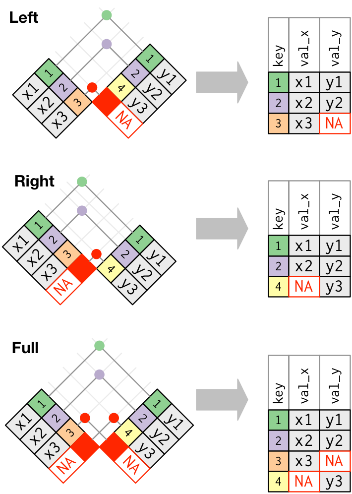
left_join:
- keeps all rows in first df (here:
flights) - adds all matching information from second df (here:
airlines); adds NAs for any observations not inairlines
. . .
Other joins:
right_join: keeps all observations in second df full_join: keeps all observations in either df
. . .
. . .
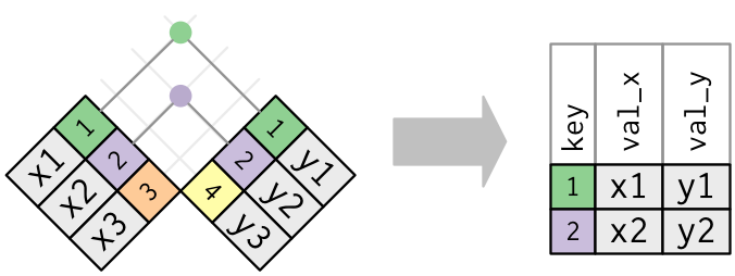
inner_join:
- takes only rows in both dfs
Recap
- Do you understand what constitutes tidy data?
- Can you identify what needs to be done to take a dataset from untidy to tidy?
- What is the difference been long data and wide data?
- Can I take long data to wide data? And wide to long?
- Can I carry out mutating joins on data?