Lab 04 - Modelling (Ans)

Author

Sean Trott

Getting Started

Load packages

library(tidyverse)
library(tidymodels)

Data

evals <- read_csv("data/evals-mod.csv")

Part 1

Exercise 1

First, we use rowwise to group evals by each row. We then use mutate to compute a new variable (bty_avg) corresponding to the average of the six beauty scores.

evals <- evals |>
  rowwise() |>
  mutate(bty_avg = mean( c( bty_f1lower, bty_f1upper,
                            bty_f2upper, bty_m1lower,
                            bty_m1upper, bty_m2upper) ))

Part 2

Exercise 2

The distribution is slightly left-skewed, i.e., many scores are on the higher side (between 4-5) with a longer tail going to the left.

This is further corroborrated by the fact that the mean is lower than the median. Given that the mean is more affected by skew than the median, this is what we’d expect with negatively skewed data.

evals |>
  ggplot(aes(x = score))+
  geom_histogram() +
  theme_bw()

`stat_bin()` using `bins = 30`. Pick better value with `binwidth`.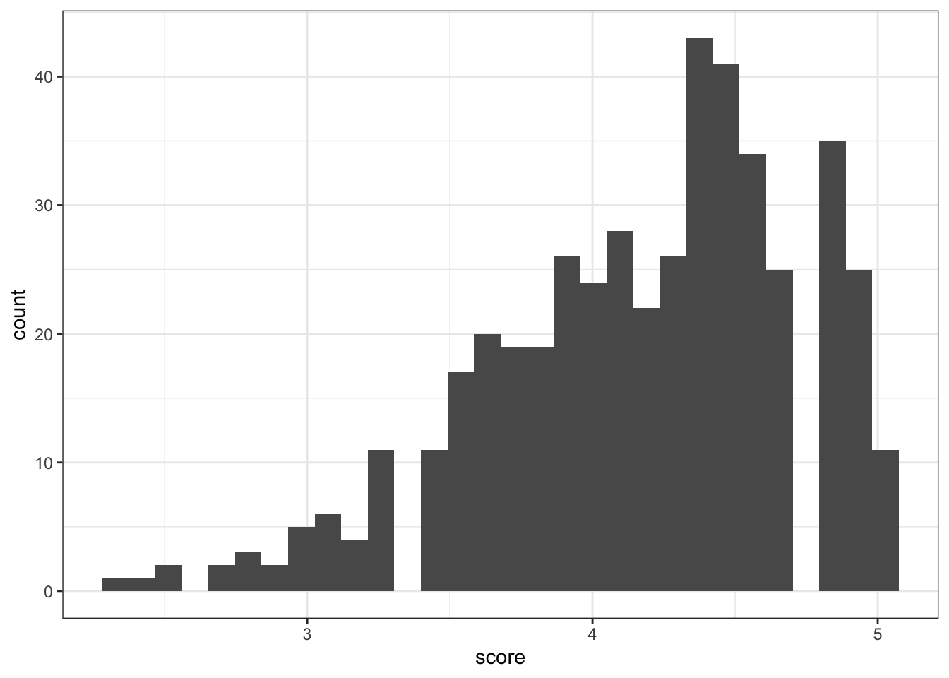

evals |>
  summarise(mean = mean(score),
            median = median(score),
            sd = sd(score))

# A tibble: 463 × 3
    mean median    sd
   <dbl>  <dbl> <dbl>
 1   4.7    4.7    NA
 2   4.1    4.1    NA
 3   3.9    3.9    NA
 4   4.8    4.8    NA
 5   4.6    4.6    NA
 6   4.3    4.3    NA
 7   2.8    2.8    NA
 8   4.1    4.1    NA
 9   3.4    3.4    NA
10   4.5    4.5    NA
# ℹ 453 more rows

Exercise 3

It seems like there’s a slight positive relationship between bty_avg and score, though it’s hard to tell given that many points overlap and form “bands” along particular values (e.g., many teachers have the same score).

evals |>
  ggplot(aes(x = bty_avg,
             y = score))+
  geom_point() +
  theme_bw()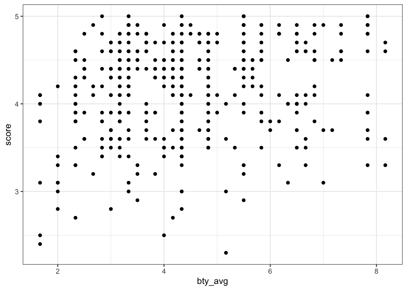

Exercise 4

One way to deal with the above is to add jitter to the plot, which reveals that certain clusters of points were either larger or smaller than initially thought. (Another apprpoach would be to change the alpha of geom_point, allowing us to detect denser clusters.)

evals |>
  ggplot(aes(x = bty_avg,
             y = score))+
  geom_jitter() +
  theme_bw()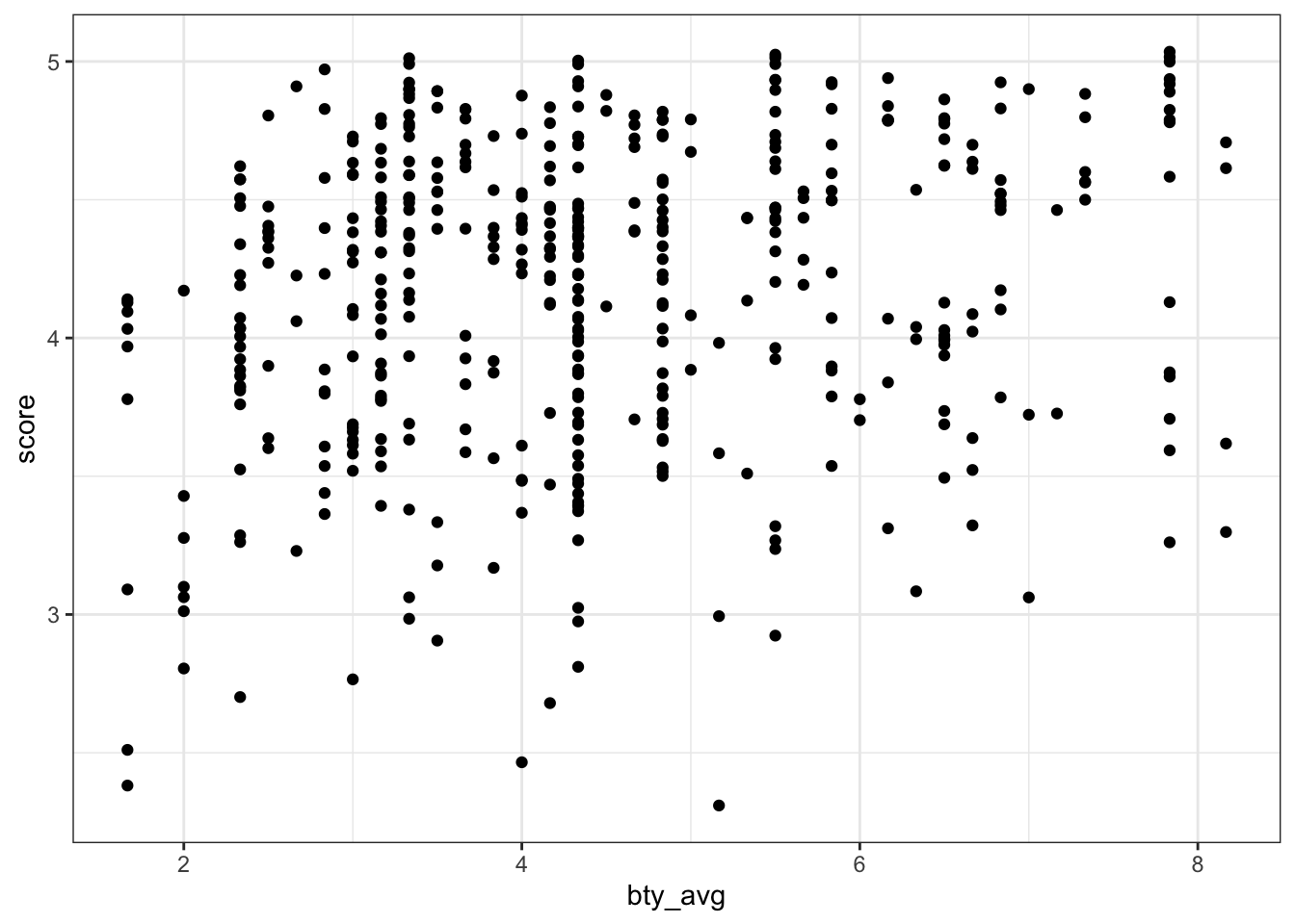

Part 3

Exercise 5

According to the model, the linear equation would be as follows:

\(\hat{y} = 3.88 + 0.07*X\)

Where \(X\) is bty_avg.

We use broom::tidy to transform the model object into a tidy dataframe.

m_bty <- linear_reg() |>
  set_engine("lm") |>
  fit(score ~ bty_avg, data = evals)

m_bty |>
  tidy() |>
  select(term, estimate)

# A tibble: 2 × 2
  term        estimate
  <chr>          <dbl>
1 (Intercept)   3.88  
2 bty_avg       0.0666

Exercise 6

evals |>
  ggplot(aes(x = bty_avg,
             y = score))+
  geom_point() +
  geom_smooth(method = "lm", 
              color = "orange",
              se = FALSE) +
  theme_bw()

`geom_smooth()` using formula = 'y ~ x'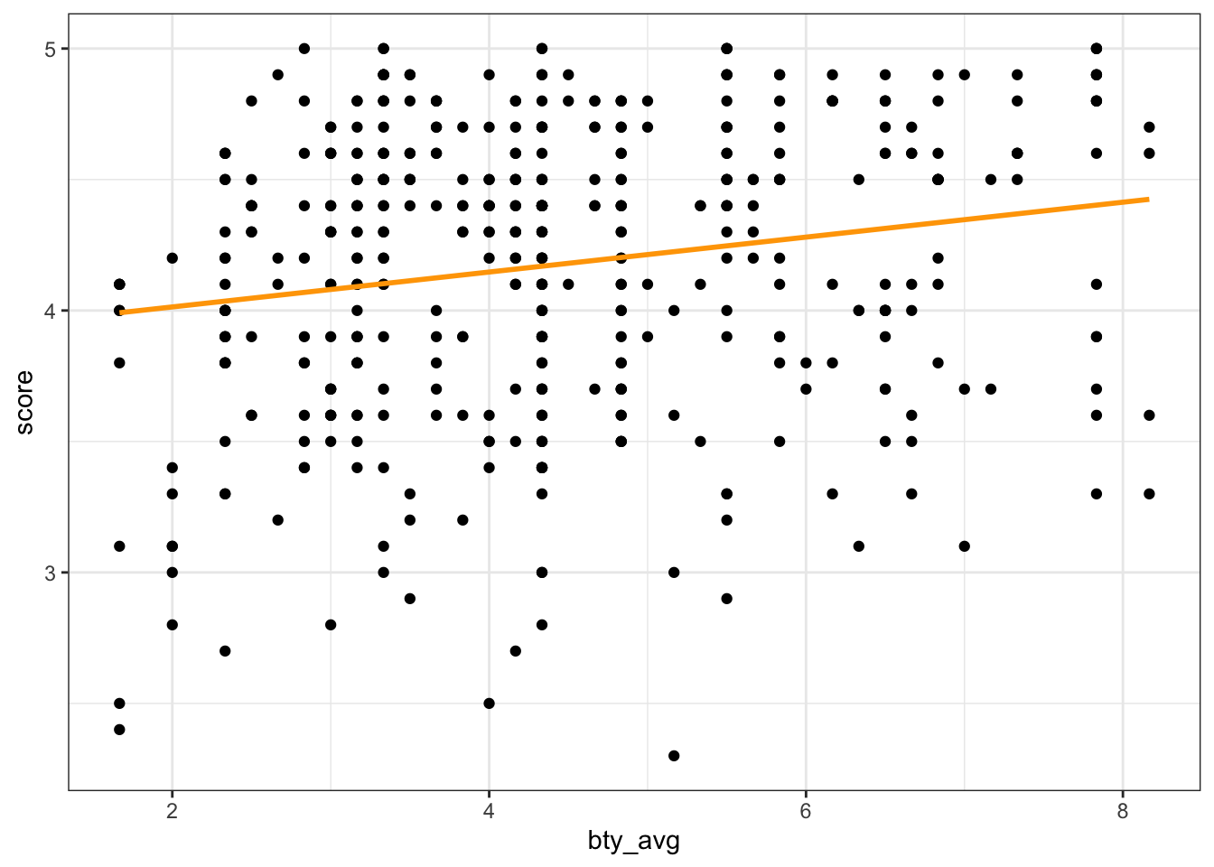

Exercise 7

Professors with higher average beauty ratings also tend to receive higher teaching scores.

The slope is approximately 0.07, which means that for every 1-unit increase in beauty rating (i.e., from 4 to 5), we can expect that a professor will receive .07 higher teaching scores (with a ~0.02 standard error).

m_bty |>
  tidy() |>
  filter(term == "bty_avg") |>
  select(term, estimate, std.error)

# A tibble: 1 × 3
  term    estimate std.error
  <chr>      <dbl>     <dbl>
1 bty_avg   0.0666    0.0163

Exercise 8

The intercept is 3.88. This is the estimated score for professors with a beauty score of 0, i.e., it is the value of \(\hat{y}\) when the regression line crosses \(x = 0\).

This may or may not make sense; given that possible beauty scores ranged from 1-6, it is a little strange to imagine a scenario where the beauty score is 0 (and it would be even stranger to imagine scenarios where the beauty scores is negative).

On the other hand, it is not inconsistent with other features of the data: the mean score, for example, is 4.17, so it makes sense that the intercept of a linear model would be slightly lower than the mean, allowing the explanatory variable to account for increases in score throughout the data.

m_bty |>
  tidy() |>
  filter(term == "(Intercept)") |>
  select(term, estimate, std.error)

# A tibble: 1 × 3
  term        estimate std.error
  <chr>          <dbl>     <dbl>
1 (Intercept)     3.88    0.0761

Exercise 9

Here, we identify the \(R^2\) of the model using glance, which identifies model-level characteristics.

The value is 0.0350, which means that our explanatory variable accounts for roughly 3.5% of the variance in our response variable.

m_bty |>
  glance() |>
  select(r.squared)

# A tibble: 1 × 1
  r.squared
      <dbl>
1    0.0350

Part 4

Exercise 10

The linear equation would be as follows:

\(\hat{y} = 4.09 + 0.142*X\)

Where \(X = 1\) for male professors and \(X = 0\) for female professors. In other words, the intercept corresponds to the mean score for female professors, while the slope tells us the difference in mean between the female average and the male average.

m_gen <- linear_reg() |>
  set_engine("lm") |>
  fit( score ~ gender, data = evals)

m_gen |>
  tidy()

# A tibble: 2 × 5
  term        estimate std.error statistic p.value
  <chr>          <dbl>     <dbl>     <dbl>   <dbl>
1 (Intercept)    4.09     0.0387    106.   0      
2 gendermale     0.142    0.0508      2.78 0.00558

Exercise 11

As specified above, the slope coefficient for the \(X\) term signifies the difference in means between male and female professors.

Exercise 12

Here, the model equation would look as follows:

\(\hat{y} = 4.28 + -0.13*X_1 + -0.145*X_2\)

Where \(X_1 = 1\) for tenure track professors and 0 for all else, and \(X_2 = 1\) for tenured professors and 0 for all else.

In other words: the intercept tells us the mean for teaching professors, and the two slope coefficients tell us the difference between that mean and the two other levels of rank.

table(evals$rank)


    teaching tenure track      tenured 
         102          108          253

m_rank <- linear_reg() |>
  set_engine("lm") |>
  fit(score ~ rank, data = evals)

m_rank |>
  tidy()

# A tibble: 3 × 5
  term             estimate std.error statistic   p.value
  <chr>               <dbl>     <dbl>     <dbl>     <dbl>
1 (Intercept)         4.28     0.0537     79.9  1.02e-271
2 ranktenure track   -0.130    0.0748     -1.73 8.37e-  2
3 ranktenured        -0.145    0.0636     -2.28 2.28e-  2

Exercise 13

Here, we use the factor command (within mutate) to reorder the levels of rank such that tenure track is the first level.

evals <- evals |>
  mutate(rank_relevel = fct_relevel(factor(rank), c("tenure track",
                                                    "teaching",
                                                    "tenured")))

Warning: There were 463 warnings in `mutate()`.
The first warning was:
ℹ In argument: `rank_relevel = fct_relevel(factor(rank), c("tenure track",
  "teaching", "tenured"))`.
ℹ In row 1.
Caused by warning:
! 2 unknown levels in `f`: teaching and tenured
ℹ Run `dplyr::last_dplyr_warnings()` to see the 462 remaining warnings.

Exercise 14

This model has the same structure as the previous model using rank, but it has reordered the levels of rank (for rank_relevel) such that tenure track is now first.

This means that the intercept should now be interpreted as the mean score for tenure track professors, and the coefficients represent the difference in means for teaching and tenured professors, respectively.

\(\hat{y} = 4.15 + 0.13*X_1 + -0.0155*X_2\)

Where \(X_1 = 1\) for teaching professors and 0 for all else; and \(X_2 = 1\) for tenured professors and 0 for all else.

We can compare tehse to the coefficients for the previous model, where teaching was the baseline: in both cases, we see that the difference between teaching and tenure track is 0.13 (just in opposite directions, depending on the baseline).

The \(R^2\) of the model is 0.0116 in both cases. In other words, the model explains approximately 1.16% of the variance in score.

m_rank_relevel <- linear_reg() |>
  set_engine("lm") |>
  fit(score ~ rank_relevel, data = evals)


m_rank_relevel |>
  tidy()

# A tibble: 3 × 5
  term                 estimate std.error statistic   p.value
  <chr>                   <dbl>     <dbl>     <dbl>     <dbl>
1 (Intercept)            4.15      0.0521    79.7   2.58e-271
2 rank_releveltenured   -0.0155    0.0623    -0.249 8.04e-  1
3 rank_relevelteaching   0.130     0.0748     1.73  8.37e-  2

m_rank_relevel |>
  glance() |>
  select(r.squared)

# A tibble: 1 × 1
  r.squared
      <dbl>
1    0.0116

Exercise 15

evals <- evals |>
  mutate(tenure_eligible = case_when(
    rank == "teaching" ~ "no",
    TRUE ~ "yes"
  ))

## Double check
table(evals$rank, evals$tenure_eligible)

              
                no yes
  teaching     102   0
  tenure track   0 108
  tenured        0 253

Exercise 16

The linear equation is as follows:

\(\hat{y} = 4.28 + -0.141*X_1\)

Where \(X_1 = 1\) for tenure eligible professors and \(X_1 = 0\) for non-tenure-eligible professors.

Thus, this means that the mean score for non-tenure-eligible professors is 4.28, and professors that are tenure eligible can expect a score that’s -0.141 lower, on average.

m_tenure_eligible <- linear_reg() |>
  set_engine("lm") |>
  fit(score ~ tenure_eligible, data = evals)

m_tenure_eligible |>
  tidy()

# A tibble: 2 × 5
  term               estimate std.error statistic   p.value
  <chr>                 <dbl>     <dbl>     <dbl>     <dbl>
1 (Intercept)           4.28     0.0536     79.9  2.72e-272
2 tenure_eligibleyes   -0.141    0.0607     -2.32 2.10e-  2

We can also calculate the \(R^2\), and we see that it is 0.0115. In other words, the model explains approximately 1.15% of the variance in score.

m_tenure_eligible |>
  glance()

# A tibble: 1 × 12
  r.squared adj.r.squared sigma statistic p.value    df logLik   AIC   BIC
      <dbl>         <dbl> <dbl>     <dbl>   <dbl> <dbl>  <dbl> <dbl> <dbl>
1    0.0115       0.00935 0.541      5.36  0.0210     1  -372.  750.  762.
# ℹ 3 more variables: deviance <dbl>, df.residual <int>, nobs <int>